When a Cohort Stops Dying

Written to a disclosure policy: errors, rankings, biases and coverage are reported as measured; totals, prices and dates finer than a year are withheld, and the two titles are pseudonyms. Every figure traces to a named table, listed at the end.

---

The question

A survival ratio for monetising users falls fast and then stops falling. What remains after a year or two is not, I think, a decaying population. It is the core who like the game — some of whom lapse and come back when a live-ops event re-engages them. That was my read of the mechanism before I measured anything, and it has a consequence: if it is right, a per-age survival ratio eventually models the wrong process, and there should be an age at which the method changes.

The composed chain asserted that age was twenty-four. Nobody had tested it. So the first question was whether the regime I described exists, and where it begins. The second, which grew out of it, was much larger: can the choice of which forecast to run, at which cohort age, for which KPI be derived from the data rather than assumed — including the choice of whether to forecast a cohort from other cohorts at the same age or from its own prior readings?

The answers came in the wrong order. The regime is real and starts early. The handover I built to exploit it is opt-in, not a default, because it inverted on the second title under the protocol that actually matters. And the grid I ran to generalise the question found something far more valuable than an age rule, which was that no age rule survives out of sample at all.

Why a deep cohort is harder to forecast than it looks

The two information sources a cohort forecast can draw on have exactly opposite availability. A three-month-old cohort has four readings of its own and twenty to thirty older siblings to learn from. A two-year-old cohort has twenty-five readings of its own and, because of the observability rule, a shrinking pool of prior cohorts that had reached that age when the forecast was made — down to a handful, and eventually none (forecast_grid__source_evidence_by_age). The counts cross at roughly age twenty on the title with fewer cohorts and roughly twenty-seven on the other. If a handover age exists anywhere, it exists here, and it is knowable in advance with no model fitted.

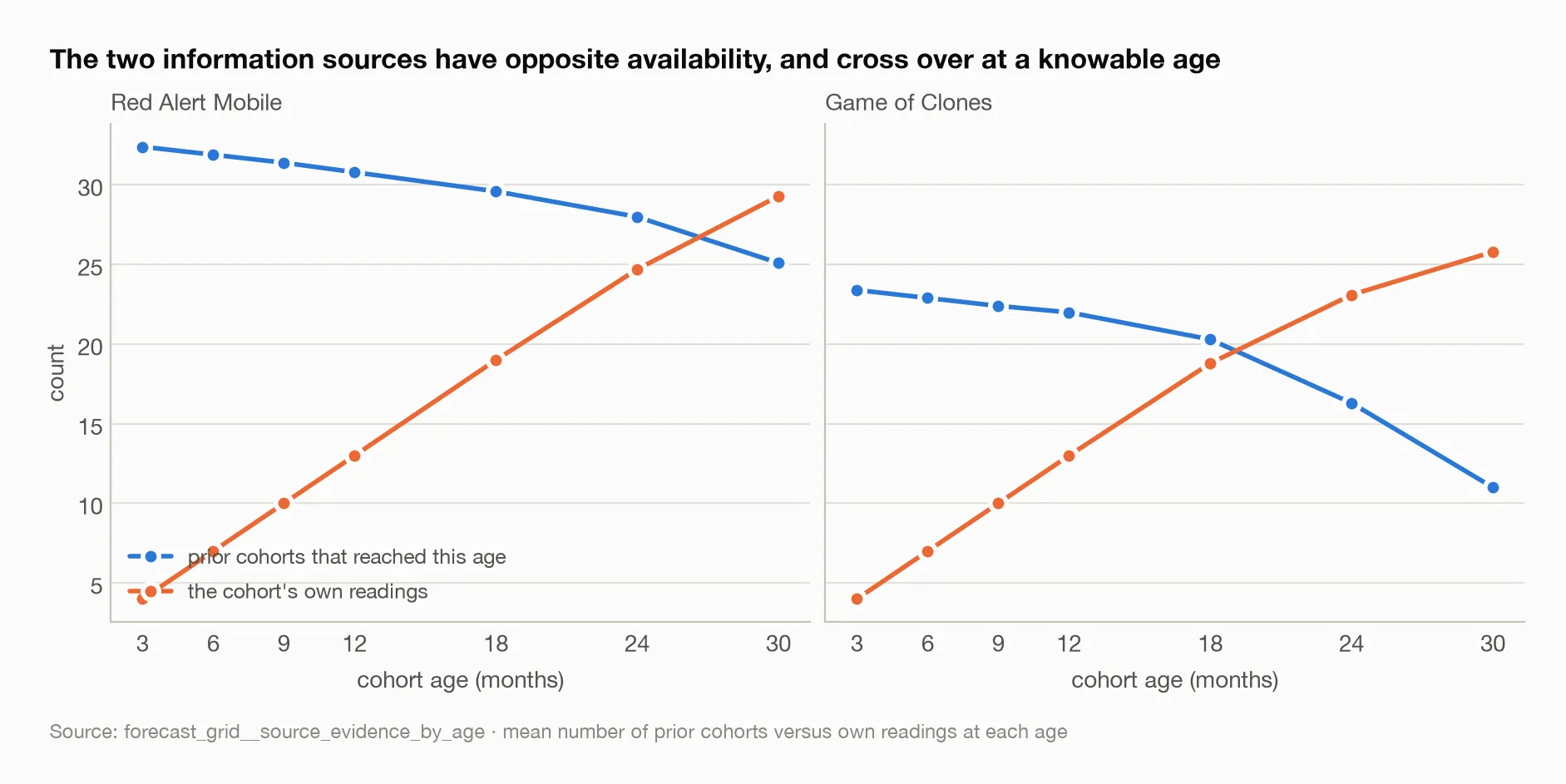
The lines cross around age twenty-seven on one title and twenty on the other, earlier on the title with fewer prior cohorts. Nothing in this chart required fitting a model or reading an outcome.

The bases matter differently at depth, too. Survival re-anchors on the age-zero value and takes the entire shape from prior cohorts — for a cohort observed for twenty months, everything after month zero is discarded. Decay chains from the most recently observed value, so all of it is carried. The advantage of carrying history should be largest where there is the most of it to throw away.

My approach

Three studies, in sequence.

Diagnose the regime. Median month-over-month decay of monetising users by cohort age, the share of cohort-months that actually grow, and cross-cohort noise, on both titles (deep_age__deep_age_diagnostics).

Sweep the handover. Five ways to carry a cohort past a switch age — per-age decay, pooled decay, carrying the last value flat, routing through active users times a conversion rate, and the incumbent per-age survival as a control — scored out of time on one fixed set of cells at every candidate switch age (deep_age__deep_age_methods). The fixed cell set is the correction to a mistake I made first: scoring each switch age only on the cells past it, so that later ages graded themselves on progressively harder subsets and early switching looked good for that reason alone.

Run the grid. Seventy-two specifications — two information sources, three bases, eight estimators, three recency windows — across six cohort-age KPIs, two titles, nine rolling origins and horizons one to twelve. Because the selection is the result, it is validated by nesting: choose on the first six origins, score on the three the choice never saw, against a floor (one shipped specification everywhere) and an oracle (the same strategy allowed to choose using the held-out data) (forecast_grid__selection_strategies).

This required a second information source that the model did not previously have. A cohort can now be extrapolated from its own prior readings, fitted on logs as either a constant decay rate or the standard flattening retention shape a(n+1)^b, or from a weighted blend of own and cross-cohort evidence.

The assumptions doing the heavy lifting

The regime can be read from the median. I diagnose it from the median month-over-month decay by age. The median hides dispersion, and a result below depends on exactly that.

A specification that wins in isolation survives composition. The grid scores cohort curves alone. A winner here still has to survive the chain, where stage errors interact. Untested.

Nine origins, three held out. Every strategy in the grid except the two at the top is separated by margins that three origins cannot resolve. The one comparison that is not close is the one I report as the finding.

The controlled comparison beats the argmax. Where the handover sweep and the grid’s winning-family map disagree — and they do, at deep ages — the sweep held the cell set fixed and asked one question, while the map is an argmax over seventy-two candidates in cells that are sometimes thin. I trust the sweep.

Where reality became inconvenient

The handover inverted under the honest protocol. Restricted to deep cells at a long horizon, switching from survival to decay wins on both titles. That is the sub-region where the mechanism lives, and I was asked — and initially intended — to make the handover the default on that evidence. Scored the way specifications are actually selected, across all cohort ages and the horizons the study plans on, it helps one title and hurts the other, and the composed chain is better end to end without it. So it is opt-in, with its evidence attached, and I reversed the instruction that prompted it on evidence gathered after it was given. The premise of that instruction also turned out to be partly an artefact: the sweep that motivated it ran before a guard on outlier decay ratios existed, and unguarded outliers were part of what it measured.

A latent bug in the decay path. A decay ratio has a tiny denominator whenever a cohort has a near-dead month, so raw ratios reach the hundreds — on the first title the largest is roughly 110. Because a decay basis chains, one such value does not add noise; it multiplies the whole remaining path. The analysis layer had always filtered these. The model module had not. The difference was invisible until a survival specification could hand over to decay, at which point it corrupted a bake-off outright. There is now a guard in both places, with a test.

The winning-family table fell out of the published report. I first wrote it as a crosstab whose column names were model families. The disclosure policy had never seen those names, so it fail-closed and silently dropped them. Published in long form, the family is a value under a recognised column. Shape the frame to the policy, not the other way round.

What the estimates actually say

The regime is real and starts early. Median monetising-user decay climbs from roughly 0.5 in the first month to about 0.95 by ages eight to twelve, then flattens and touches 1.0. The share of cohort-months that grow rises from zero to between a third and a half by age two. Cross-cohort noise roughly doubles over the same span. Both titles (deep_age__deep_age_diagnostics). Past the first year these cohorts are not decaying so much as fluctuating around a slowly eroding core — but the flattening begins around age eight to twelve, not twenty-four.

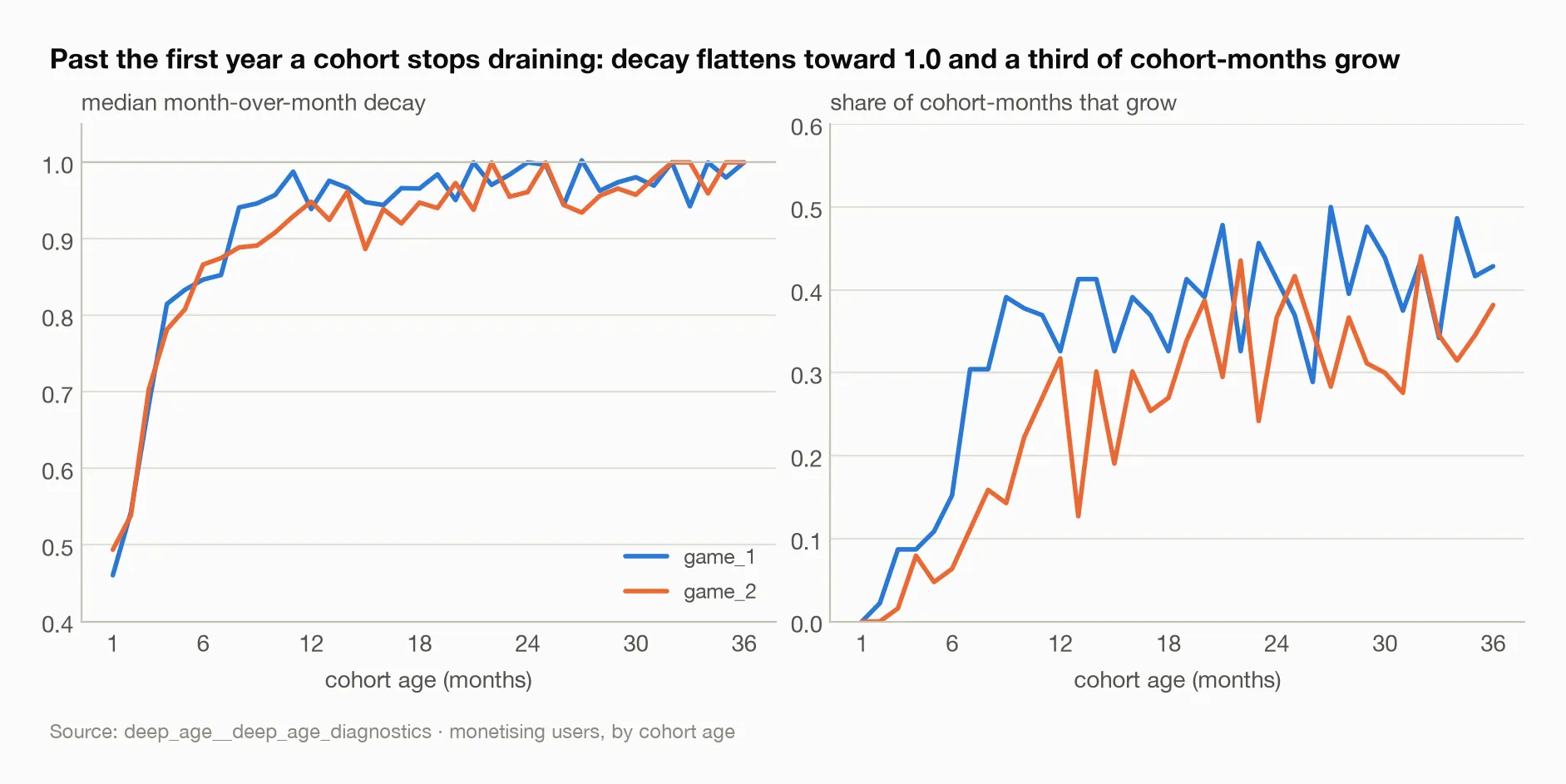
Both titles trace the same shape: a steep climb in the decay ratio over the first eight to twelve months, then a plateau at or near one. On the right, the share of cohort-months that grow rises from zero to a third or more — a population that is fluctuating, not draining.

Per-age decay beats per-age survival at depth, and the earlier the switch the better. On one fixed cell set, the incumbent per-age survival scores 0.675 on the first title and 0.316 on the second; switching to per-age decay scores 0.397 at a switch age of six and 0.265 at nine (deep_age__deep_age_methods).

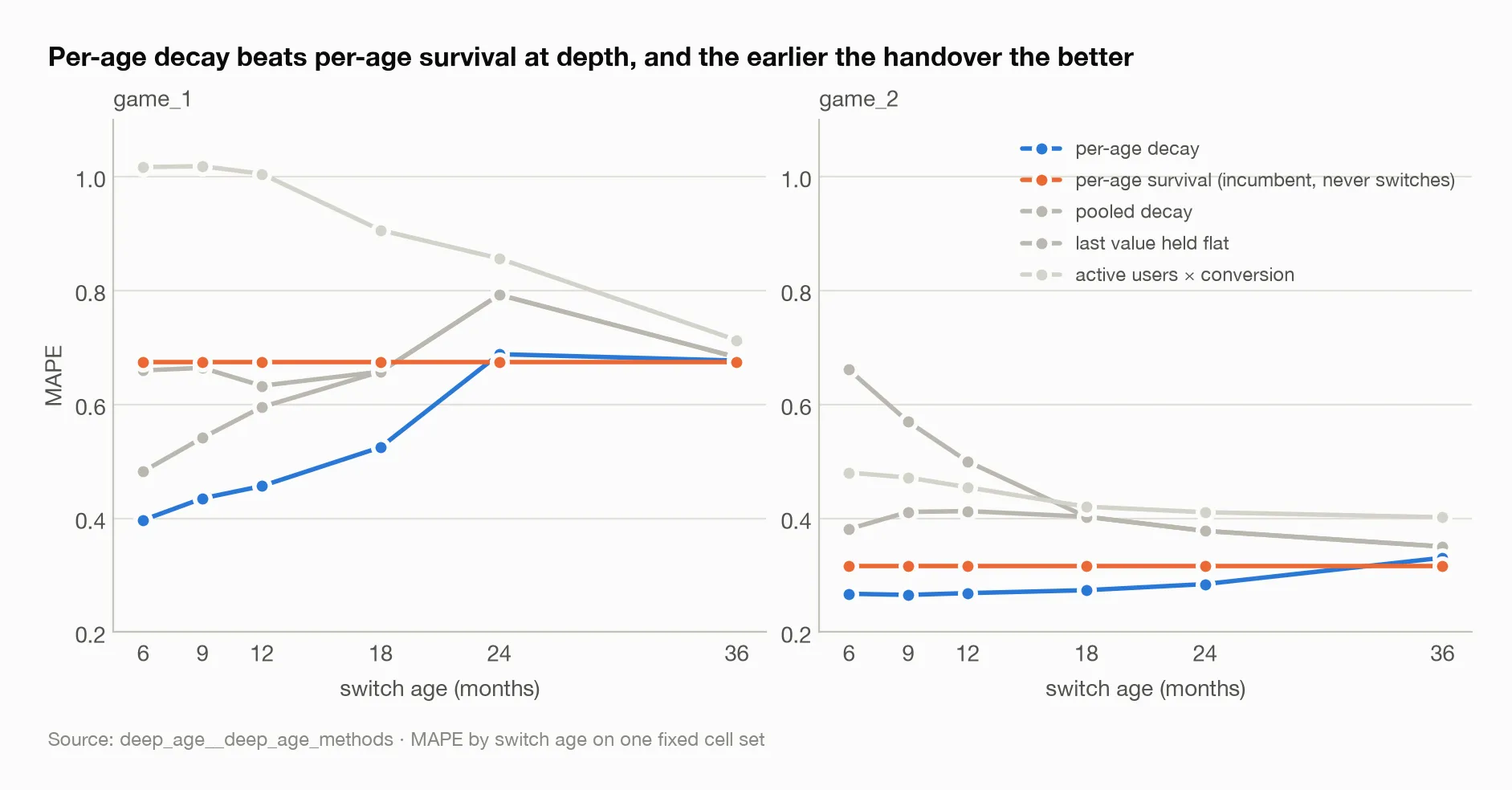
The orange line is the control: it never switches, so it is flat. The blue line is below it at every switch age on both titles, lowest at the earliest switch, and converges on it by age thirty-six. The gray lines are the alternatives, all worse.

The advantage decays monotonically as the switch is pushed later; by age thirty-six the two bases have converged. Routing through active users times a conversion rate loses on both titles — 0.713 to 1.018 on the first — which is the revenue-per-user lesson again: composing two forecasts multiplies two errors, and a conversion rate is not stable enough to carry the product. Carrying the last value flat is also poor despite median decay sitting near 1.0 at depth, because cohorts scatter around that flat level rather than sitting on it.

This resolves an apparent contradiction with the stage bake-off, which selects survival for monetising users. That comparison is dominated by young cohorts at short horizons — precisely where survival should win, because there is little history to discard and the age-zero anchor is close. Both results are correct. They answer different questions, and the age-dependent rule they jointly imply runs opposite to the one shipped: survival for young cohorts and short horizons, decay from roughly age six to nine onward.

Selecting per metric pays. Selecting per age does not. Held-out mean MAPE by strategy, averaged over twelve metric-account pairs (forecast_grid__selection_strategies):

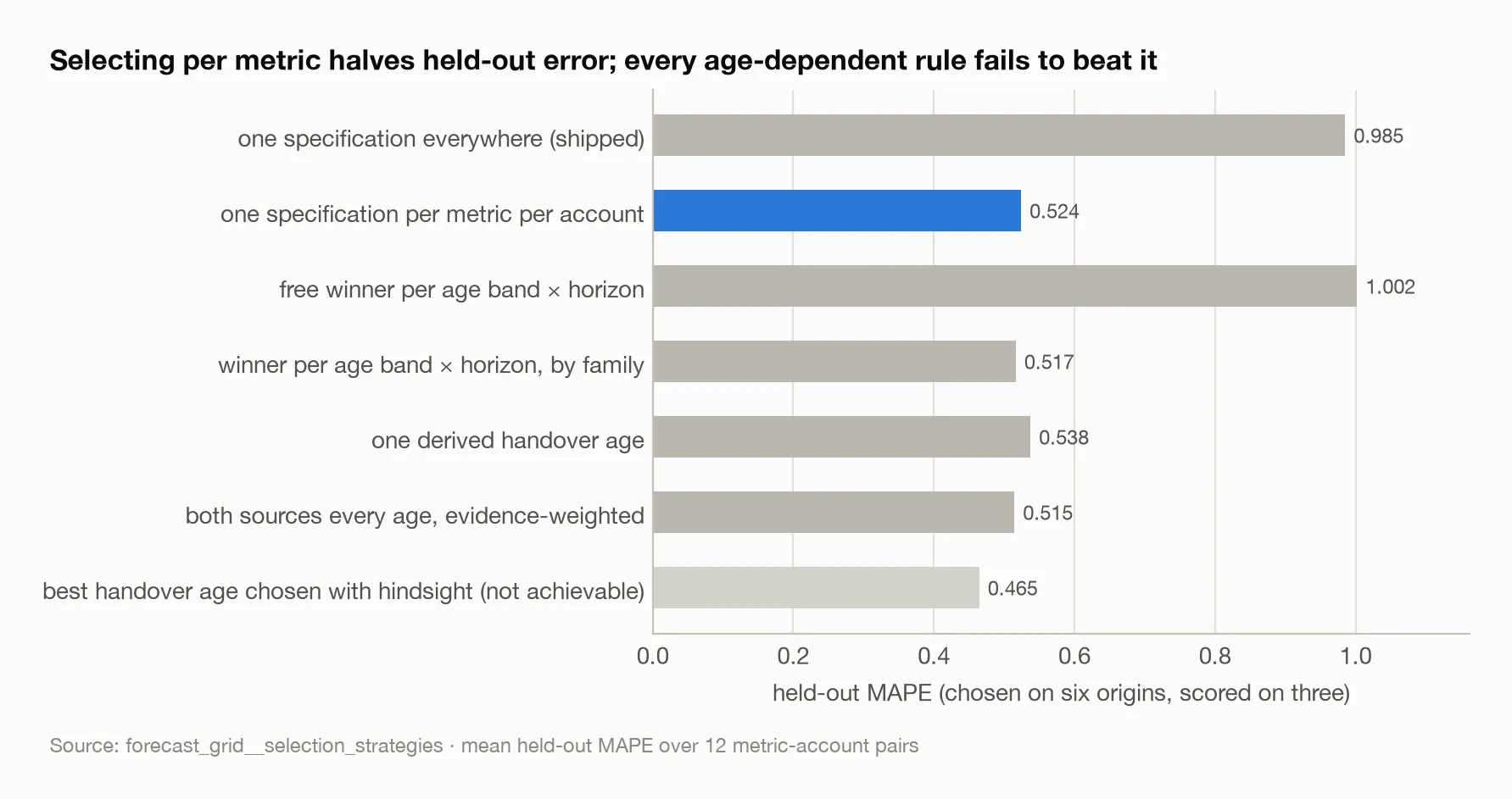
The blue bar is the only strategy that clearly beats the shipped floor, and it has no age-dependence in it. The four age-dependent strategies below it land within a few thousandths of it or, in one case, worse than choosing nothing. The pale bar at the bottom is the oracle, which is not achievable and bounds what any age rule could recover.

The one that pays has no age-dependence in it at all. Choosing a single specification per metric per account cuts held-out error from 0.985 to 0.524 — better on ten of twelve metric-account pairs, and the largest improvement for the effort anywhere in this study. It needs no new modelling, only the discipline of running the selection out of time per metric rather than carrying one default.

Every route to age-dependence fails. The free per-cell winner is the worst strategy tested — worse than choosing nothing — because a thin cell picks a specification that does not generalise, and one pair blows out by an order of magnitude. Coarsening to family granularity contains that and lands a wash. A single derived handover age, with one degree of freedom instead of twenty, is worse than not doing it, and picks “never” on six of twelve pairs.

The oracle row is why this is a negative result rather than a null one. Allowed to pick the handover with hindsight on the held-out data, it reaches 0.465. So roughly a seventh of the error genuinely is age-structured — and none of it is recoverable from data available at forecast time. The age-dependence is real and not identifiable. At this sample size, the cost of estimating where the handover goes exceeds what the handover is worth.

The map says something anyway. Counting winning families across all metrics, horizons and both titles (forecast_grid__winning_family_by_age), the cross-cohort decay basis dominates at ages zero to five, the cohort’s own power-curve fit takes over from age six through twenty-three, and cross-cohort survival and the own exponential fit lead past twenty-four. Chain off the most recent reading while the curve is steep and the cohort has no history; hand over to the cohort’s own shape once it has one; fall back to a cross-cohort curve at depths where an own fit is extrapolating furthest past its data. Read it as a mechanism, not a rule — the strategies chart above is the measurement of what happens when you try to act on it.

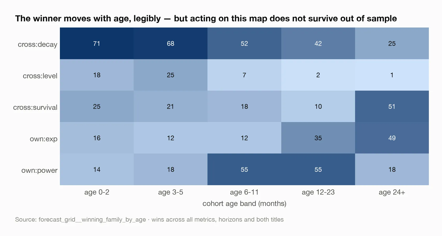
Darker is more wins. Cross-cohort decay dominates the youngest bands, the cohort’s own power-curve fit takes over from age six to twenty-three, and cross-cohort survival and the own exponential fit lead past twenty-four. The structure is real; the strategies chart above is what it is worth.

Three things fell out that were not the question (forecast_grid__selection_winners). The basis is an account property, not a metric property: every cross-cohort winner on one title is survival and every one on the other is decay, six metrics each, no exceptions — and it is n = 2, and this study has twice published corrections that looked this clean and failed a second-account test. A median of prior cohorts beats the shipped recency-weighted mean on ten of eleven pairs where they differ, which is consistent with a shared calendar shock loading recency weights onto exactly the shocked months. And quantities that drain want an exponential while quantities that flatten want a power curve — every own-curve winner on revenue is a constant decay rate, every own-curve winner on a user count is the flattening retention shape. Two processes, separated by the grid without being told to look. The own-curve source is the globally best specification on six of twelve pairs, which makes it the substantive addition here — more so than the age question that motivated building it.

What I would change next time

Adopt per-metric selection, or decide not to. The shipped default is the selected winner on none of twelve pairs and loses to the per-metric choice on ten. Adopting it means the chain carries a selection table rather than a default, which changes how it is configured and deployed. It is the largest known unexploited improvement in the study, and it is a design decision.

Run the sweep on revenue. The handover result is for monetising users only. The chain forecasts revenue directly, and this does not transfer without testing.

Sweep the recency window and the horizon. Neither was varied. A twelve-month horizon with a six-cohort window is one point in a plane.

Score the winners through the composition. A specification that wins alone has not yet won.

The broader lesson

I set out to find an age and found a distribution of ages I could not afford to estimate. That is a more useful thing to know. The oracle row says the structure is there; the strategies say it costs more to locate than it returns. “There is nothing there” and “there is something there you cannot afford to estimate” call for different next steps, and it is worth building the oracle to know which one you have.

The handover taught me about the difference between a mechanism and a default. The regime is real; I could see it in the diagnostics on both titles. Winning in the region where the mechanism lives is not the same as winning under the protocol the model is actually selected with, and I had to reverse a decision I had already argued for once the second protocol was run. I would rather record that than smooth it over.

And the grid’s by-products remind me that the most valuable output of a large experiment is often orthogonal to its motivating question. I built a second information source to answer an age question. The age question came back negative. The source is the best specification on half the pairs.

Sources

Every figure above traces to one of these tables:

• deep_age__deep_age_diagnostics — decay, growing share and noise by age
• deep_age__deep_age_methods — the handover sweep on a fixed cell set
• forecast_grid__source_evidence_by_age — prior-cohort versus own-history counts by age
• forecast_grid__selection_strategies — the nested-origin strategy comparison
• forecast_grid__winning_family_by_age — winning families by age band
• forecast_grid__selection_winners — the per-metric-per-account winners

forecastingcohort analysismodel selectionretentiondecay